Problem statement

On Shopify, we have exactly 100 sneaker shops, and each of these shops sells only one model of shoe. We want to do some analysis of the average order value (AOV). When we look at orders data over a 30 day window, we naively calculate an AOV of $3145.13. Given that we know these shops are selling sneakers, a relatively affordable item, something seems wrong with our analysis.

• Think about what could be going wrong with our calculation. Think about a better way to evaluate this data.
• What metric would you report for this dataset?
• What is its value?

Analysis comprehension

What information do we seek?

Well, since the average order value of a 30-day window is being reported, it means that we want information on the average amount spent each time a customer places an order.

AOV =RN where R = Revenue, and N = no of orders.

1. Given that sneakers are affordable items, an AOV of $3,145.13 is intuitively absurd, but only through analysis can we confirm this. Some possible contenders for such an AOV are

• Insufficient analytics (e.g. wrong formulas being utilized)
• Presence of outliers in terms of order amount
• a small/wrongly calculated N value and large R

Analytics approach

Our analytics will depend on the depth of information we seek, but say we just need a basic perfomance metric that informs on how much customers spend each time they place an order, then we could

• Perform exploratory data analysis (EDA) to evaluate the presence of outliers
• Depending on the outcome of EDA, we could report the mean or median with confidence interval

Let’s begin the analytics

# Load the necessary packages 
required_packages <- c("tidyverse", "data.table", "gsheet",
                       "Hmisc", "psych", "lubridate",
                       "rmarkdown", "knitr")

packageCheck <- lapply(required_packages, FUN = function(x) {
  if(!require(x, character.only = TRUE)) {
    install.packages(x, dependencies = TRUE)
    library(x, character.only = TRUE)
  }
})

# Import the data 
shopify_sales <- gsheet2tbl("https://docs.google.com/spreadsheets/d/16i38oonuX1y1g7C_UAmiK9GkY7cS-64DfiDMNiR41LM/edit#gid=0")

Let us begin by getting summary statistics on the pooled data as it pertains to AOV

# Get basic summary statistics on the data
psych::describe(shopify_sales[, c("order_amount", "total_items")])

##              vars    n    mean       sd median trimmed    mad min    max  range
## order_amount    1 5000 3145.13 41282.54    284  287.39 174.95  90 704000 703910
## total_items     2 5000    8.79   116.32      2    1.88   1.48   1   2000   1999
##               skew kurtosis     se
## order_amount 16.67   279.51 583.82
## total_items  17.06   288.96   1.65

Immediately, we observe things such as the huge standard deviation relative to mean for both the order amount and total items i.e. 

• Order amount: 3145.13±41282.54
• Total items: 8.79±116.32

The relatively large deviations from the mean immediately inform us high variance in the data set and possible presence of outliers. The standard error for the order amount is thus high and informs that the mean is likely an inaccurate representation of the true mean.

2. What metric would you report for this dataset?

In this scenario, it is more appropriate to report the median as opposed to the mean because the median is more robust against outliers. We can thus report a value of $284, albeit the presence of outliers in the data.

Let us do some more exploratory data analysis, following separation of the order amount into a subset excluding the outliers.

# Make box-plot to visualize basis summary content of data 
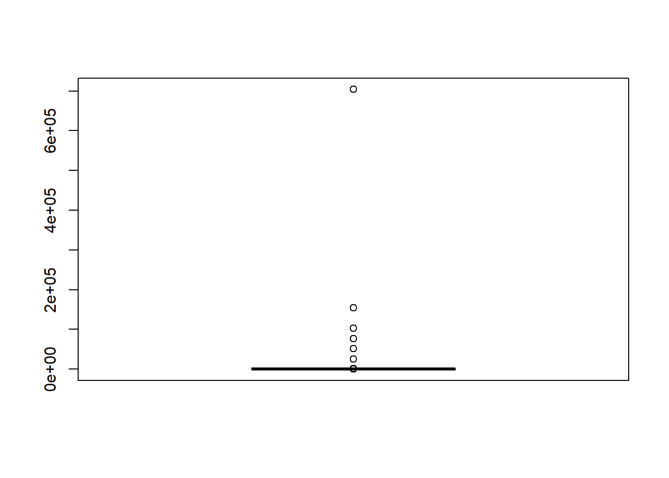
order_amount_boxplot_full <- boxplot(shopify_sales$order_amount, plot = T)

Immediately we see that outliers are indeed present, and the scale of these outliers relative to our data is so much that we are unable to evaluate the non-outlier subset of data within our data set. On that note, let us do another visualization without the outliers, but not discard the outliers though, as they may be interesting components of our data that we may want to further evaluate.

# Store outliers
order_amount_outliers <- order_amount_boxplot_full$out
describe(order_amount_outliers)

##    vars   n     mean       sd median  trimmed    mad min    max  range skew
## X1    1 141 101407.6 225491.5   1056 39221.84 474.43 735 704000 703265 2.25
##    kurtosis       se
## X1     3.17 18989.81

# Get order amounts not in outliers 
order_amount_no_outliers <- shopify_sales$order_amount[-which(shopify_sales$order_amount %in% order_amount_outliers)]
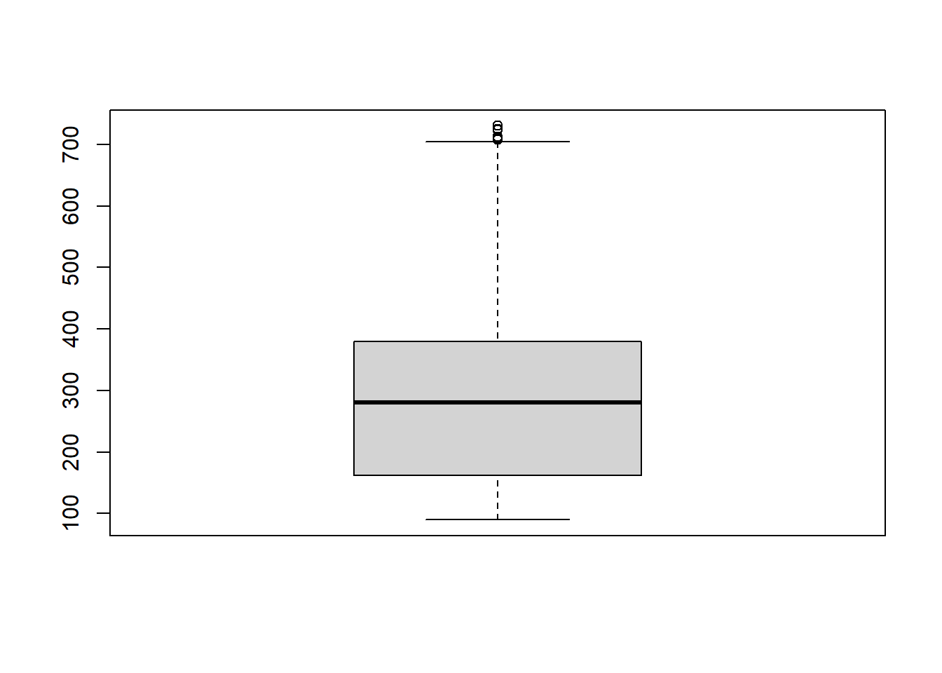
describe(order_amount_no_outliers)

##    vars    n   mean     sd median trimmed    mad min max range skew kurtosis
## X1    1 4859 293.72 144.45    280  279.23 167.53  90 730   640 0.73    -0.17
##      se
## X1 2.07

# Let us make another plot showing the distribution of the data 
boxplot(order_amount_no_outliers)

Let up apply some more intuition before reporting metrics on our analysis. Firstly, it is mentioned that we seek data over 30 days, so let us confirm that we do indeed have 30 days worth of data in our data set

shopify_sales$created_at <- ymd_hms(shopify_sales$created_at)
max(shopify_sales$created_at) - min(shopify_sales$created_at)

## Time difference of 29.99127 days

Ok, we are good to go.

Next, what percentage of our data are outliers; a confirmation that we aren’t discarding much of our data.

cat("Outlier percentage of data:", (length(order_amount_outliers)/nrow(shopify_sales)) * 100)

## Outlier percentage of data: 2.82

cat("\nWe are reporting based on", length(order_amount_no_outliers), "no of transactions in 30 days, i.e.", length(order_amount_no_outliers)/nrow(shopify_sales) * 100, "percent of our data")

## 
## We are reporting based on 4859 no of transactions in 30 days, i.e. 97.18 percent of our data

3. What is its value?

cat("In 30 days of sales, the metrics are: ",
    "\n1) The mean value when outliers are included =",
    describe(shopify_sales$order_amount)$mean,
    "\n2) the mean value when outliers are excluded =",
    describe(order_amount_no_outliers)$mean, 
    "\n3) the median value when outliers are included =", 
    describe(shopify_sales$order_amount)$median,
    "\n4) the median value when outliers are excluded =",
    describe(order_amount_no_outliers)$median)

## In 30 days of sales, the metrics are:  
## 1) The mean value when outliers are included = 3145.128 
## 2) the mean value when outliers are excluded = 293.7154 
## 3) the median value when outliers are included = 284 
## 4) the median value when outliers are excluded = 280

Any of metrics 2 to 4 will be appropriate to return, in this case I will proceed with options 1 or 3, depending on whom the information will be presented to. If it is an in-house presentation, I can inform that the AOV was 3,145.13,butthisincluded141transactionsthatarelikelyoutliersgiventheirorderamountsrelativetoothertransactionthatoccurred.becauseitconsidersallthedatagiven.Forageneralpresentation,Icanreportavalueof284.00 because it contains all transactions, yet, it is not heavily impacted by outliers.

SQL Query Challenge

1. How many orders were shipped by Speedy Express in total?

• In total, there were 54 orders shipped by Speedy Express

Code logic:

• We want to know how many orders were shipped by one of the shipping companies, Shippers. This means that firstly, we have to query the database to access the table containing the different shipping companies and their IDs, and select the information pertaining the company whose information we seek, i.e. Speedy Express.

• Next, we go a level up to find the number of orders that were shipped by Speedy Express. This means we have to access the orders table within the database and find the linkage parameter between the Shippers table and the Orders table. Upon finding this linkage parameter, we perform our computation on the Orders table, querying to find the requested information, and next, we link to the Shippers table using the linkage parameters, reporting only the required information.

Code chunk:

SELECT COUNT(*) AS "Speedy_Express_Order_Count" 
FROM Orders
WHERE Orders.ShipperID = 
(
  SELECT ShipperID 
  FROM Shippers 
  WHERE ShipperName = "Speedy Express"
  );

2. What is the last name of the employee with the most orders?

• The last name of the employee with the most orders is Peacock

Code logic:

• Much like the previous question, we have to find linkage parameters contained in the different tables within the database. However, compared to the previous example, other SQL functions such JOIN, GROUP BY, ORDER BY, and LIMIT need to be called at different stages of our query to ensure that at each step, the appropriate information being sought is provided.

Code chunk:

SELECT Employees.LastName
FROM Employees
LEFT JOIN Orders
ON Orders.EmployeeID = Employees.EmployeeID
GROUP BY Orders.EmployeeID
ORDER BY COUNT(Orders.EmployeeID) DESC
LIMIT 1;

3. What product was ordered the most by customers in Germany?

• Boston Crab Meat was the product ordered the most by customers in Germany

Code logic:

• Once again, logic takes the helm as we have to find linkage parameters contained in the different tables within the database, albeit with several linkages connecting the different tables.

Code chunk:

SELECT 
Products.ProductName, SUM(OrderDetails.Quantity) AS Total_orders, Customers.Country
FROM Products
JOIN OrderDetails ON OrderDetails.ProductID = Products.ProductID
JOIN Orders ON Orders.OrderID = OrderDetails.OrderID
JOIN Customers ON Customers.CustomerID = Orders.CustomerID
WHERE Customers.Country = "Germany"
GROUP BY Products.ProductName
ORDER BY Total_orders DESC
LIMIT 1;